Perceptron
A perceptron is a binary classification algorithm modeled after the functioning of the human brain—it was intended to emulate the neuron. The perceptron, while it has a simple structure, has the ability to learn and solve very complex problems.

Multilayer Perceptron
A multilayer perceptron (MLP) is a group of perceptrons, organized in multiple layers, that can accurately answer complex questions. Each perceptron in the first layer (on the left) sends signals to all the perceptrons in the second layer, and so on. An MLP contains an input layer, at least one hidden layer, and an output layer

The Perceptron Learning Process
The Perceptron Learning Process happens through following steps:
1. Takes the inputs which are fed into the perceptrons in the input layer, multiplies them by their weights, and computes the sum.
2. Adds the number one, multiplied by a “bias weight”. This is a technical step that makes it possible to move the output function of each perceptron (the activation function) up, down, left and right on the number graph.
3. Feeds the sum through the activation function—in a simple perceptron system, the activation function is a step function.
4. The result of the step function is the output.

From Perceptron to Deep Neural Network
A multilayer perceptron is quite similar to a modern neural network. By adding a few ingredients, the perceptron architecture becomes a full-fledged deep learning system:
Activation functions and other hyperparameters —a full neural network uses a variety of activation functions which output real values, not boolean values like in the classic perceptron. It is more flexible in terms of other details of the learning process, such as the number of training iterations (iterations and epochs), weight initialization schemes, regularization, and so on. All these can be tuned as hyperparameters.
Backpropagation—a full neural network uses the backpropagation algorithm, to perform iterative backward passes which try to find the optimal values of perceptron weights, to generate the most accurate prediction.
Advanced architectures—full neural networks can have a variety of architectures that can help solve specific problems. A few examples are Recurrent Neural Networks (RNN), Convolutional Neural Networks (CNN), and Generative Adversarial Networks (GAN).
Understanding Backpropagation in Neural Networks
What is Backpropagation and Why is it Important?
After a neural network is defined with initial weights, and a forward pass is performed to generate the initial prediction, there is an error function which defines how far away the model is from the true prediction. There are many possible algorithms that can minimize the error function—for example, one could do a brute force search to find the weights that generate the smallest error. However, for large neural networks, a training algorithm is needed that is very computationally efficient. Backpropagation is that algorithm—it can discover the optimal weights relatively quickly, even for a network with millions of weights.
How Backpropagation Works
1. Forward pass—weights are initialized and inputs from the training set are fed into the network. The forward pass is carried out and the model generates its initial prediction.
2. Error function—the error function is computed by checking how far away the prediction is from the known true value.
3. Backpropagation with gradient descent—the backpropagation algorithm calculates how much the output values are affected by each of the weights in the model. To do this, it calculates partial derivatives, going back from the error function to a specific neuron and its weight. This provides complete traceability from total errors, back to a specific weight which contributed to that error. The result of backpropagation is a set of weights that minimize the error function.
4.Weight update—weights can be updated after every sample in the training set, but this is usually not practical. Typically, a batch of samples is run in one big forward pass, and then backpropagation performed on the aggregate result. The batch size and number of batches used in training, called iterations are important hyperparameters that are tuned to get the best results. Running the entire training set through the backpropagation process is called an epoch.

Backpropagation in the Real World
In the real world, you will probably not code an implementation of backpropagation, because others have already done this for you. You can work with deep learning frameworks like Tensorflow or Keras, which contain efficient implementations of backpropagation, which you can run with only a few lines of code.
Understanding Neural Network Activation Functions
Activation functions are central to deep learning architectures. They determine the output of the model, its computational efficiency, and its ability to train and converge after multiple iterations of training.
What is a Neural Network Activation Function?
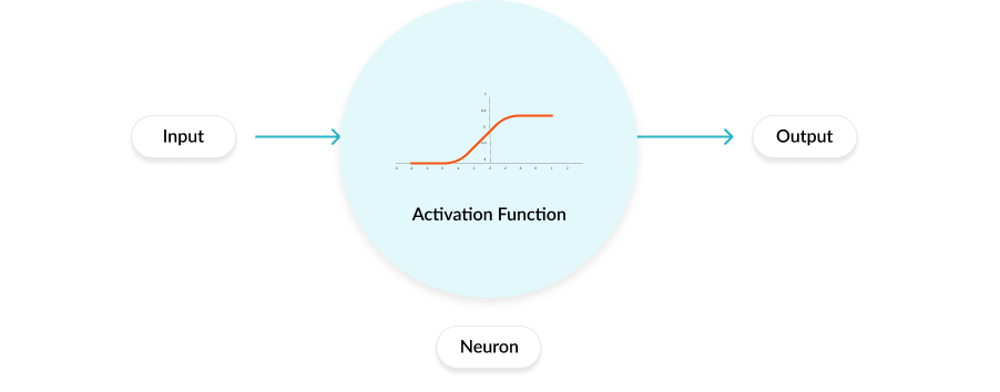
An activation function is a mathematical equation that determines the output of each element (perceptron or neuron) in the neural network. It takes in the input from each neuron and transforms it into an output, usually between one and zero or between -1 and one. Classic activation functions used in neural networks include the step function (which has a binary input), sigmoid and tanh. New activation functions, intended to improve computational efficiency, include ReLu and Swish.

Role of the Activation Function
In a neural network, inputs, which are typically real values, are fed into the neurons in the network. Each neuron has a weight, and the inputs are multiplied by the weight and fed into the activation function. Each neuron’s output is the input of the neurons in the next layer of the network, and so the inputs cascade through multiple activation functions until eventually, the output layer generates a prediction. Neural networks rely on nonlinear activation functions—the derivative of the activation function helps the network learn through the backpropagation process

7 Common Activation Functions (More details at 7 Types of Neural Network Activation Function)
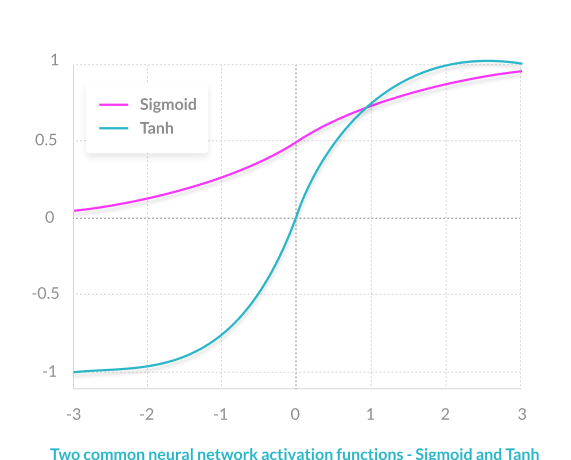
The sigmoid function has a smooth gradient and outputs values between zero and one. For very high or low values of the input parameters, the network can be very slow to reach a prediction, called the vanishing gradient problem.
The TanH function is zero-centered making it easier to model inputs that are strongly negative strongly positive or neutral.
The ReLu function is highly computationally efficient but is not able to process inputs that approach zero or negative.
The Leaky ReLu function has a small positive slope in its negative area, enabling it to process zero or negative values.
The Parametric ReLu function allows the negative slope to be learned, performing backpropagation to learn the most effective slope for zero and negative input values.
Softmax is a special activation function use for output neurons. It normalizes outputs for each class between 0 and 1, and returns the probability that the input belongs to a specific class.
Swish is a new activation function discovered by Google researchers. It performs better than ReLu with a similar level of computational efficiency.


